Bitcoin and other crypto currencies are known for their volatility and ability to make monstrous moves seemly out of nowhere. The purpose of this little investigation is to see if these moves can provide any meaningful insight into the direction BTC will go in the next several days.
Please note none of this article or any other article i publish is to be considered financial advice.
First off is going to be some code to setup our experiments and to prep us for the various filters to come.
# howitzer is my own python library used it interface with some of the other downtocrypto related libraries
from howitzer.util.trading import *
from howitzer.util.stats import *
from enum import Enum
from datetime import datetime
import matplotlib.pyplot as plt
 # I will find some way to zip and send this data hopefully
chart = chartFromDataFiles("../HistoricData/Cbp/BTC-USD", datetime(2016,1,1), datetime(2021,10,31))["daily"]
# create a list of just the percentage of the candles
all_percents = list(map(lambda candle : candle.percent, chart.candles))
# Get some basic information
minPercent = min(all_percents)
maxPercent = max(all_percents)
print(minPercent, maxPercent)
-37.264189567966945 27.20197964577091
# Create groups to bucket the number of time a particular percent shows up
buckets = []
labels = []
positiveVnegative = [0, 0]
lowest = round(minPercent)
highest = round(maxPercent)
for i in range(lowest, highest):
    labels.append(i)
    buckets.append(0)

for i in range(len(all_percents)):
    percent = round(all_percents[i])
    buckets[percent - lowest -1] =  buckets[percent - lowest - 1] + 1
    if all_percents[i] < 0:
        positiveVnegative[0]+=1
    elif all_percents[i] > 0:
        positiveVnegative[1]+=1
# Graph frequency of each percentage
fig = plt.figure()
ax = fig.add_axes([0,0,1,1])
ax.bar(labels,buckets)
plt.show()
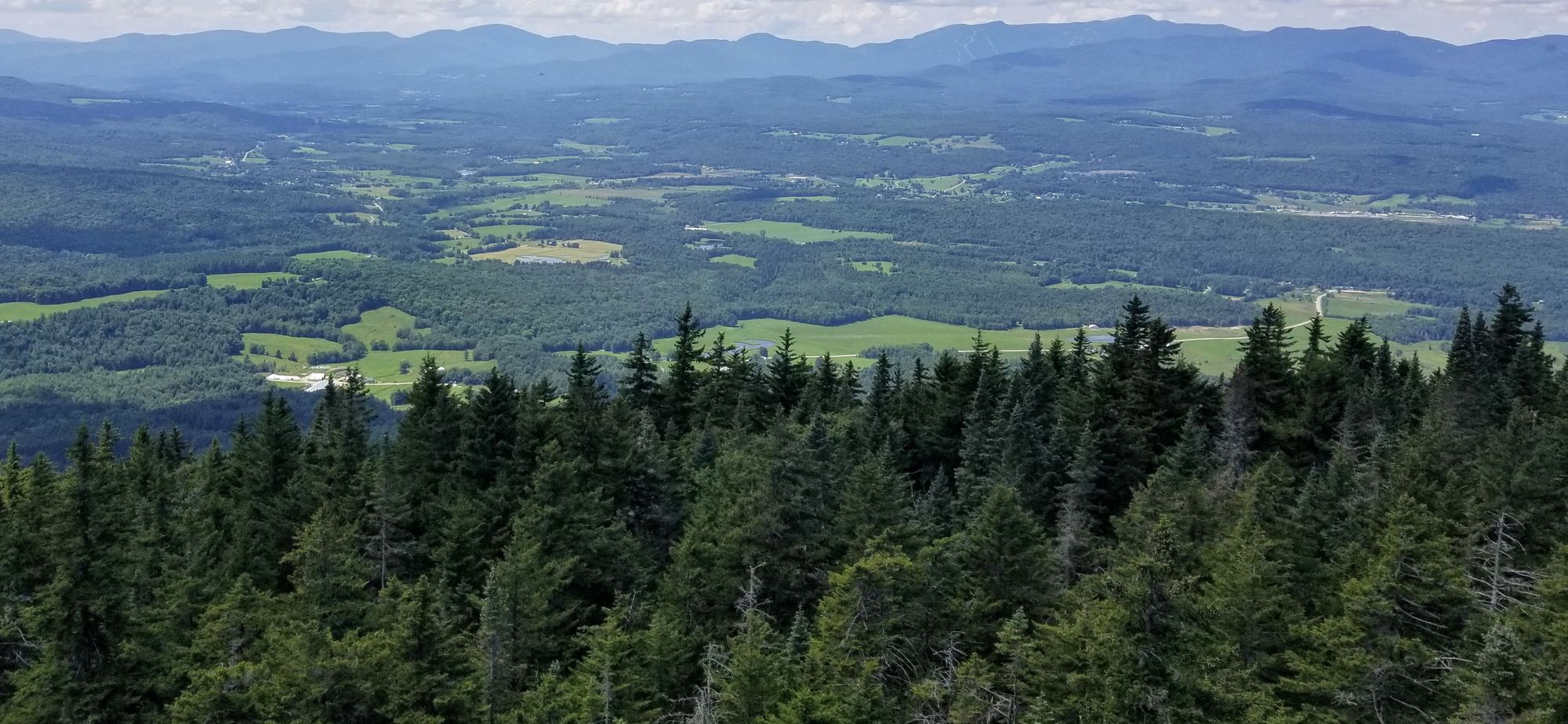
Observation
The distribution of the movement range of bitcoin on any given day seems to be a standard bell curve, unfortunately centered around -1%. This is an issue as +/- 1% is not typically enough of a movement to overcome fees associated with trading and even the bias towards the -1% range isn't going to overcome the fees of buying and selling plus the leverage fees for most retail accounts.
So, what qualifies as a "large" move.
For our purposes we are going to consider anything outside of the mean +/- 2 standard deviations as that will be outside of 95% of the normal range of the data.
standardDeviation = stddev(all_percents)
mean = average(all_percents)
twoStd = mean + 2 * standardDeviation
twoStdNegative = mean - 2 * standardDeviation
print(f"The standard deviation  is {standardDeviation}")
print(f"The average movement in a day is {mean}")
print(f"The top of the two standard deviations {twoStd}")
print(f"The bottom of the two standard deviations {twoStdNegative}")
The standard deviation  is 4.058865449751024
The average movement in a day is 0.32561980472018714
The top of the two standard deviations 8.443350704222235
The bottom of the two standard deviations -7.792111094781861
Note
In the above we established and saved the values we will want to investigate throughout the experiment.
Now for more setup code.
# Function to append percent change x days ahead
def lookForward(candles, index, distance, _list):
    if index + distance < len(candles):
        close = candles[index].close
        temp = round(100*(candles[index+distance].close-close)/close,1)
        _list.append(temp)

# Function to get the highest high that occurs from the inspected candle to x days ahead
def lookForwardHigh(candles, index, distance, _list):
    if index + distance < len(candles):
        start = index+1
        highs =  list(map(lambda candle : candle.high, candles[start:start+distance]))
        high = max(highs)
        close = candles[index].close
        temp = round(100*(high-close)/close,1)
        _list.append(temp)

# Function to get the lowest low that occurs from the inspected candle to x days ahead
def lookForwardLow(candles, index, distance, _list):
    if index + distance < len(candles):
        start = index+1
        lows =  list(map(lambda candle : candle.low, candles[start:start+distance]))
        lowestLow = min(lows)
        close = candles[index].close
        temp = round(100*(lowestLow-close)/close,1)
        _list.append(temp)

# Bring it all together and deliver it to the masses
def Experiment(filterMethod=lambda a : True, compareMethod=lookForward,timeSteps=[5,10,20,30]):
    sampleCount = 0
    candlesToLoopThrough = chart.candles.copy()
    #candles are loaded in gdax (coinbase pro) order, most recent first so they need reversed to do a sequencial run through
    candlesToLoopThrough.reverse()

    catagories = []
    for step in timeSteps:
        catagories.append({"distance":step, "values":[]})

    for i in range(len(candlesToLoopThrough)):
        candle = candlesToLoopThrough[i]
        close = candle.close

        if filterMethod(candle):
            sampleCount +=1
            for cat in catagories:
                compareMethod(candlesToLoopThrough, i, cat["distance"], cat["values"])

    print(f"Number of Samples in data {sampleCount}")
    lables = []
    values = []
    for cat in catagories:
        x = cat["distance"]
        lables.append(f"{x} Days Out")
        values.append(average(cat["values"]))
    fig = plt.figure()
    ax = fig.add_axes([0,0,1,1])
    ax.bar(lables, values)
    plt.show()
Note
In the above code there are several things we do to lay the groundwork for our experiments.
LookForward is a function that takes in an array of candles and determines the increase in price from a specific candle's close to the close of a specific candle some predetermined time in the future. This is going to be a useful metric for us to look at and judge the performance of a given filter or entry.
# run the sample case to see what happens on every day of buying BTC
Experiment()
Experiment(compareMethod=lookForwardHigh)
Experiment(compareMethod=lookForwardLow)
Number of Samples in data 2131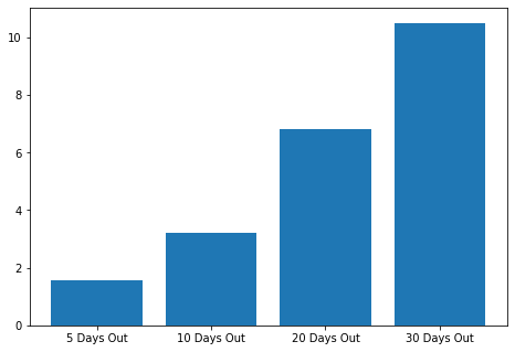
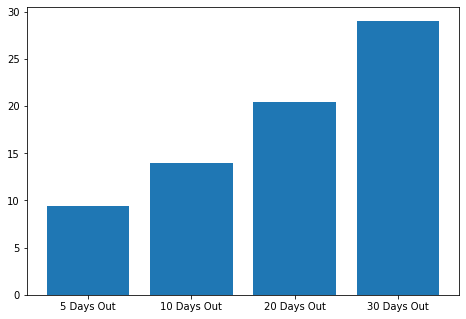
Observation
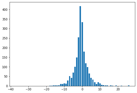
These are our baselines, the numbers to beat for all filters and potential entries going forward.
The first graph shows the average percent change from the close of any given day to the close 5, 10, 20 and 30 days out.
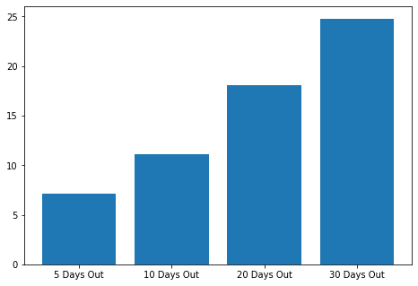
The second graph shows the average percent difference between the close of any given day and the highest high recorded 5, 10, 20, and 30 days out.
The third and final graph shows the average percent difference between the close of any given day and the lowest low recorded 5, 10, 20 and 30 days out.
So, what does this all mean?
Well first off BTC is biased to the upside and on average you are going to be up 10% 30 days in the future having bought any given day in the past between January 2016 and October 2021.
# run the sample case to see what happens after a two standard deviations move
Experiment(filterMethod=lambda candle : candle.percent > twoStd)
Experiment(filterMethod=lambda candle : candle.percent > twoStd, compareMethod=lookForwardHigh)
Experiment(filterMethod=lambda candle : candle.percent > twoStd, compareMethod=lookForwardLow)
Number of Samples in data 68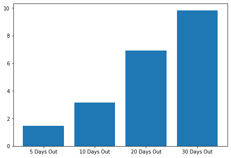
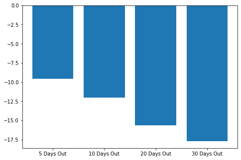
Observation
The first graph shows the average percent change from the close of a day with a percent move 2 standard deviations above the mean to the close 5, 10, 20 and 30 days out. This matches very closely to the percent change on any given day.
The second graph shows the average percent difference between the close of a day with a percent move 2 standard deviations above the mean and the highest high recorded 5, 10, 20, and 30 days out. This metric outperformed the average potentially yielding some alpha to be taken advantage of.
The third and final graph shows the average percent difference between the close of a day with a percent move 2 standard deviations above the mean and the lowest low recorded 5, 10, 20 and 30 days out. Here the metric underperforms the average which could be an issue for the signal's use in a strategy.
Both experiments have a similar closing price change 5, 10, 20, and 30 days out suggesting a return to the status quo after the event. The difference in the high and lows suggests some short-term volatility after the event that is shaken out as time goes on.
There could be an advantage there, so I want to investigate the same two situation but 1, 2, 3, 4, and 5 days out from the event to see if the alpha is in the short term rather than the long term.
# run the sample case to see what happens on every day of buying BTC with 1, 2, 3, 4 and 5 day time frames
Experiment(timeSteps=[1,2,3,4,5])
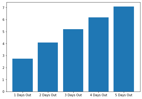
Experiment(compareMethod=lookForwardHigh,timeSteps=[1,2,3,4,5])
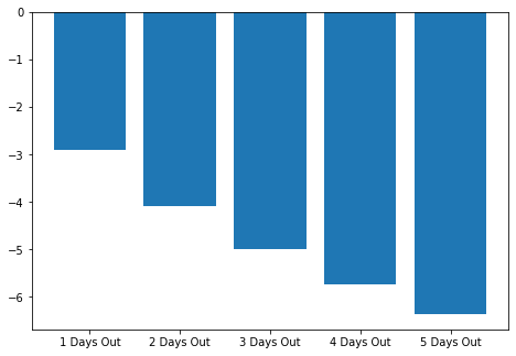
Experiment(compareMethod=lookForwardLow,timeSteps=[1,2,3,4,5])
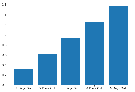
Observation
Again we are creating a baseline to compare our potential signals too.
The linear nature of our grpahs paints a very clear picture of BTC's slight upward bias along with the steady nature of the volatality over time. Note on graph 2 and 3 how the highs and lows for 1, and 2 days our are near mirrors of one another.
It is predicted that the short term volatality will be much different after a 2 standard devation move.
# run the sample case to see what happens after a two standard deviations move with 1, 2, 3, 4 and 5 day time frames
Experiment(filterMethod=lambda candle : candle.percent > twoStd, timeSteps=[1,2,3,4,5])
Experiment(filterMethod=lambda candle : candle.percent > twoStd, compareMethod=lookForwardHigh, timeSteps=[1,2,3,4,5])
Experiment(filterMethod=lambda candle : candle.percent > twoStd, compareMethod=lookForwardLow, timeSteps=[1,2,3,4,5])
Number of Samples in data 68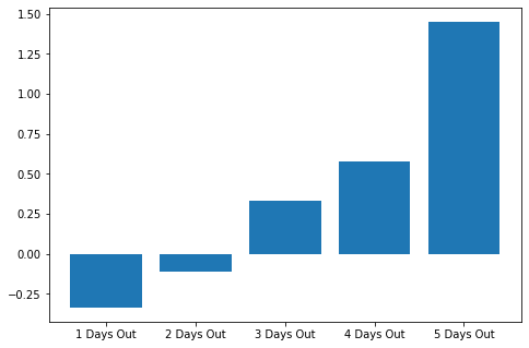
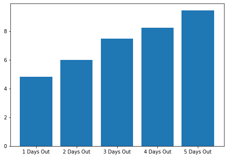
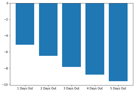
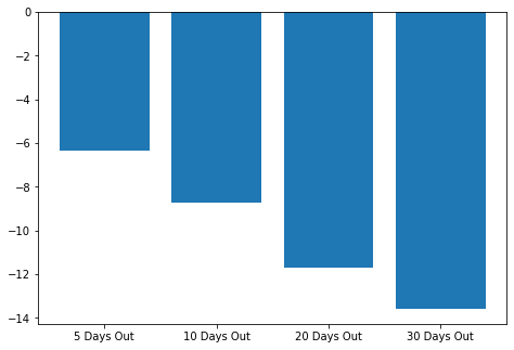
Observation
Well, this is different.
Right out of the gate graph 1 which is the average close after the event shows our first negative value both 1 and 2 days after the close of the large move candle.
Graphs 2 and 3 paint a very clear picture of the volatility faced shortly after such events. If the average close is just below -0.25% but the average high is over 4% and the average low is below -4% the swings much larger then on an average day in the BTC world.
The only question that remains is what happens first the high or the low.
Strategy Brain Storming
As I've mentioned before when I enter a trade, I enter knowing exactly what conditions will cause me to get out of the trade. I've used trailing stops, time stops, moving averages as well as basic stops and targets. So, if we enter on a move after a day where the price action is two standard deviations above the mean price movement, based on this data, when should we get off the wild ride? As mentioned before the long-term advantage does not appear to be there so I am thinking something in the ballpark of 72 hours tops. Using the daily close as a signal is out as that underperforms the return of buying on any given day. So, a stop and a target it is.
Looking at the data the first thought that comes to mind is a stop and target of +/- 4%. This is within the average range that occurs after these large moves. This also begs the question of what do we want to do at the end of the day? In my personal opinion if the trade has not exited by the end of the day, I would want to exit the trade for now. We could change this but since our initial stops and targets are based on one day after the large move our trade could be considered invalidated after that.
Our Bot's First Go
For test parameters I used market orders with fees of 0.5% both ways on the same data tested here.
After running it through my back-testing platform that I use for the rest of my trading i got a report on the strategy's performance and let me tell you it was terrible.
Things already started out difficult for us as having a stop and target of the same size means our risk reward ratio is 1 and once fees are considered it becomes less than 1. In order for a strategy with a risk reward ratio less than one to be profitable it needs over a 60% win rate.
Report
- Win Rate: 34%
- PnL: -114%
- Average Winner: 3% (-1% of target likely due to fees)
- Average loser: 4% (not -5% likely due to the loses that were triggered on end of day)
- Average Time in Winner: 10 hours
- Average Time in Loser: 12 hours
Not good we may need to go back to the drawing board.
Brainstorming Round 2: Scalping
So, we know there is volatility after these candles and that the swings are quite large. Can we capture just the slightest of moves and achieve a high win rate? Let’s aim for a 2% target and keep the 4% stop to give us some breathing room to see how that changes thing. I know it’s a bit of a stretch but it’s worth trying.
Report
- Win Rate: 54%
- PnL: -102%
- Average Winner: 1% (-1% of target likely due to fees)
- Average loser: 4.61%
- Average Time in Winner: 3 hours
- Average Time in Loser: 11 hours
Better but still untradeable. I have one last tool in my tool belt, and I haven't used it in a while.
AI anyone?
Aim for Over Optimized
A while ago I developed a means of which to use genetic optimization to help tweak strategies. It was an undertaking that took months, and I haven't really used it since as I was having issues with what measure to grade the variants on, and it would tend to focus down and eliminate trades to be severely the dataset. I think we will still have over fitting here, but it won't eliminate trades as I have seen in the past so let’s see what we can do.
I am only going to optimize the stop and targets and I am going to have it maximize the gains of the strategy.
I am using a population of 16 organisms and going to go through 10 generations and use a mutation rate of 0.2 the whole time.
The top 3 organisms of one generation will carry over to the next generation.
Since it’s all in Java Script it will take way too long so I will start it before I go to bed and check it when I get home from work.
Results
- Target: 2.75%
- Stop: 9%
Report
- Win Rate: 53.7%
- PnL: -60%
- Average Winner: 1.9%
- Average loser: -4.1%
- Average Time in Winner: 7 hours
- Average Time in Loser: 22 hours
Better than before but still not tradeable.
I may give it another parameter of how many days to hold for and let it optimize that as well but this article is already getting extremely long so it will have to wait until next time.
Conclusion
The hope was that trading after one of these large upward moves would provide some statistical edge when going long BTC-USD. It is not clear that this is not the case and that after these moves price is not biased upward and could even be biased downward. Even when exits were optimized using genetic learning there still was no available edge.
But have no fear as all is not lost. We can still look at what happened after large downward moves as well as possibly predicting these types of moves. Perhaps one of those will provide a reasonable edge to trade.
Hope you enjoyed this more in-depth article, as I rather enjoyed writing it.
One final reminder that none of this is to be considered financial advice and is to be looked at for entertainment purposes only.
Thank for stopping by, hope you come back soon!