Massively Meaningful Moves or Mediocre Market Signals: Part Two

I’ll get it out of the way right away...

None of this or anything else on my blog or social media accounts is to be considered financial advice. Everyone is responsible for their own actions and there are plenty of qualified professionals who are more than happy to help.

Based on the previous look into significantly large moves in the crypto universe it was determined that the environment after a larger (greater than two standard deviations) up move provides little to no alpha or trading advantage.

I did leave off on a cliff hanger regarding the last AI run through I had planned. So, without further ado here was the outcome.

Results

Target: 42%
Stop: -33%
Max Time in Trade: 72 hours

Report

Win Rate: 62%
PnL: 67%
Average Winner: 7.8%
Average loser: -4.1%
Average Time in Winner: 113 hours
Average Time in Loser: 113 hours

Analysis

While this may look good on paper it’s really a rather poor strategy. The equity curve spikes up sharply in early 2017 then slowly falls back over the next three and a half years. Not a system I want to be trading. But it is cool to see the genetic learning optimize a strategy. In this case it found it was best to wait exactly 113 hours after the signal to see to get the best result. In the trading history it never once hit the stop and target only using the 113 hours wait time to exit. Running the strategy on other pairs yielded a similar result.

I may come back and look at how various filters effect the bot in the later future, but it’s time to look forward.

Recap

Last time we looked at the use of large price moves upwards providing bullish signals for BTC-USD. The best result that was discovered was the AI grown start discussed above. This we are going to examine the long opportunities presented by large down moves. Why long only? Currently I lack the capital to receive the leverage necessary to take short positions ever since Kraken changed their rules regarding leverage.

So let’s start by setting our environment back up almost exactly as we did last time.

# howitzer is my own python library used it interface with some of the other downtocrypto related libraries
from howitzer.util.trading import *
from howitzer.util.stats import *
from enum import Enum
from datetime import datetime
import matplotlib.pyplot as plt
plt.rcParams['figure.figsize'] = [10, 5]

 # I will find some way to zip and send this data hopefully
chart = chartFromDataFiles("../../overlord/HistoricData/Cbp/BTC-USD", datetime(2016,1,1), datetime(2021,10,31))["daily"]

# create a list of just the percentage of the candles
all_percents = list(map(lambda candle : candle.percent, chart.candles))

# Get some basic information
minPercent = min(all_percents)
maxPercent = max(all_percents)
print(minPercent, maxPercent)

standardDeviation = stddev(all_percents)
mean = average(all_percents)
twoStd = mean + 2 * standardDeviation
twoStdNegative = mean - 2 * standardDeviation
print(f"The standard deviation  is {standardDeviation}")
print(f"The average movement in a day is {mean}")
print(f"The top of the two standard deviations {twoStd}")
print(f"The bottom of the two standard deviations {twoStdNegative}") # our focus for this endevor

-37.264189567966945 27.20197964577091
The standard deviation  is 4.058865449751024
The average movement in a day is 0.32561980472018714
The top of the two standard deviations 8.443350704222235
The bottom of the two standard deviations -7.792111094781861

# Function to append percent change x days ahead
def lookForward(candles, index, distance, _list):
    if index + distance < len(candles):
        close = candles[index].close
        temp = round(100*(candles[index+distance].close-close)/close,1)
        _list.append(temp)
        
# Function to get the highest high that occurs from the inspected candle to x days ahead
def lookForwardHigh(candles, index, distance, _list):
    if index + distance < len(candles):
        start = index+1
        highs =  list(map(lambda candle : candle.high, candles[start:start+distance]))
        high = max(highs)
        close = candles[index].close
        temp = round(100*(high-close)/close,1)
        _list.append(temp)
        
# Function to get the lowest low that occurs from the inspected candle to x days ahead
def lookForwardLow(candles, index, distance, _list):
    if index + distance < len(candles):
        start = index+1
        lows =  list(map(lambda candle : candle.low, candles[start:start+distance]))
        lowestLow = min(lows)
        close = candles[index].close
        temp = round(100*(lowestLow-close)/close,1)
        _list.append(temp)

# Bring it all together and deliver it to the masses
# Making 1, 2, 3, and 4 part of the default 
def Experiment(filterMethod=lambda a : True, compareMethod=lookForward,timeSteps=[1, 2, 3, 4, 5, 10, 20, 30]):
    sampleCount = 0
    candlesToLoopThrough = chart.candles.copy()
    #candles are loaded in gdax (coinbase pro) order, most recent first so they need reversed to do a sequencial run through
    candlesToLoopThrough.reverse()

    catagories = []
    for step in timeSteps:
        catagories.append({"distance":step, "values":[]})
    
    for i in range(len(candlesToLoopThrough)):
        candle = candlesToLoopThrough[i]
        close = candle.close
        
        if filterMethod(candle):
            sampleCount +=1
            for cat in catagories:
                compareMethod(candlesToLoopThrough, i, cat["distance"], cat["values"])
    
    print(f"Number of Samples in data {sampleCount}")
    lables = []
    values = []
    for cat in catagories:
        x = cat["distance"]
        lables.append(f"{x} Days Out")
        values.append(average(cat["values"]))
    fig = plt.figure()
    ax = fig.add_axes([0,0,1,1])
    ax.bar(lables, values)
    plt.show()

# Let us re-establish the baseline
# run the sample case to see what happens on every day of buying BTC
Experiment()
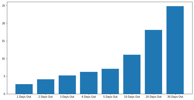
Experiment(compareMethod=lookForwardHigh)
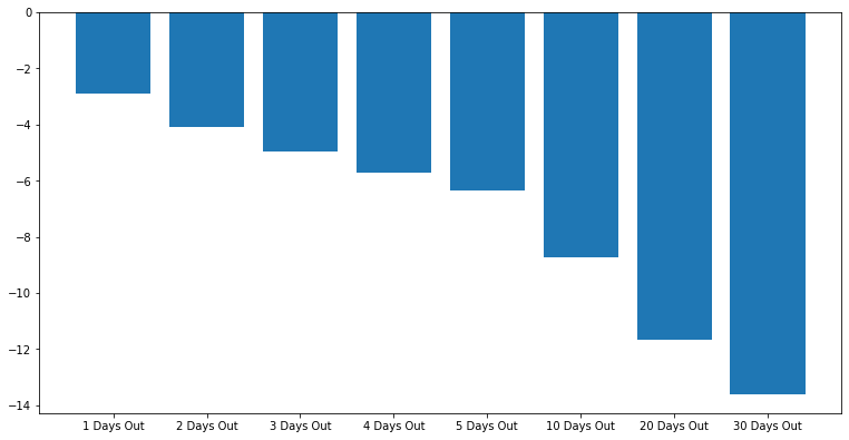
Experiment(compareMethod=lookForwardLow)

Number of Samples in data 2131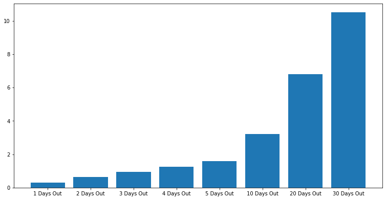

Observation

As mentioned in our previous article these are our baselines. If our signals provide higher highs, lower lows or higher closes compared to buying on any given day there is more likely to be an edge that can be exploited by us or AI optimization.

So, let’s get right into it.

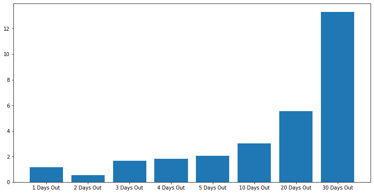
# run the sample case to see what happens after a two standard deviations move
Experiment(filterMethod=lambda candle : candle.percent < twoStdNegative)
Experiment(filterMethod=lambda candle : candle.percent < twoStdNegative, compareMethod=lookForwardHigh)
Experiment(filterMethod=lambda candle : candle.percent < twoStdNegative, compareMethod=lookForwardLow)

Number of Samples in data 58

Observation

Wow this is interesting.

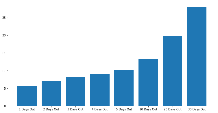
As before the first graph shows the average percent change from the close of the day with a percent move less than two standard deviations from the mean for 1, 2, 3, 4, 5, 10, 20 and 30 days out.

Graph 2 is the average highest high after a change two standard deviations below the mean for 1, 2, 3, 4, 5, 10, 20, and 30 days out.

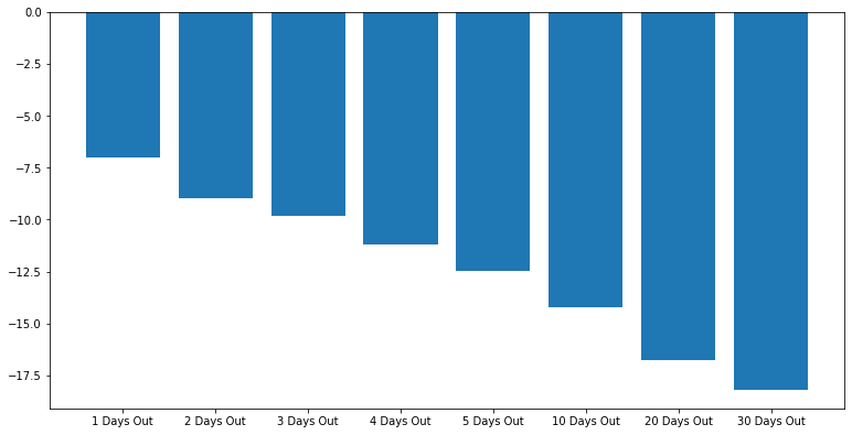
Graph 3 is the average lowest low 1, 2, 3, 4, 5, 10, 20 and 30 days out.

So as with large moves there seems to be a large increase in volatility shortly after the event. Notice the increase in the scale in the average lowest low and highest high. This is like the volatility noticed during the previous look at the upward moves, however it is larger in scale. One could argue fear being a more actionably emotion could lead towards this volatility spike. Noticeably the lowest lows are lower on all look forward tests.

The average closing price lags after these events until the 20-day mark where it then seems to outperform by a percent or two on the 30-day mark. This suggests either a consolidation period or a downward move occurs most of the time after such an event. This could be another strike against simply taking a long position immediately after such an event.

The concerning factor here is the drastic increase in the average lowest low value. This means any reasonable stop we pick is likely to get hit. The lowest low is also greater in magnitude then the highest high until around the 20-day mark as well. This means there is usually more downward pressure for some time after these events.

But none of this is going to stop us from trying!

Strategy Brain Storming

If the average move upward is slightly over 5%, I think it is fair to use this as a target. I will start with a 2.5% stop and see how that does. I'm not going to dice too far into this as given the current information I really don't want to be involved in trades around this type of event unless they provide a massive advantage.

Results

Win Rate: 44%
PnL: -100%
Average Winner: 3.8%
Average loser: -6%
Average Time in Winner: 25 hours
Average Time in Loser: 16 hours

Well, that went about as bad as it could have. Due to only being able to account for price action every 15 seconds the wild price movements resulted in slippage of both the entries and exits further securing the profit and loss of the trades. One thing i did find interesting was that the losers held for roughly 5 hours less than the winners on average. Something I want to explore in the AI portion of this investigation.

AI

So, this time i want to give the bot another parameter to optimize. Last time it ignored the stop and target and simply used the time in the trade to determine its exit. What if we also gave it a delay to enter the trade? So, after the signal Give it up to 5 days to enter and a max of being in the trade for 5 days. This could be really interesting and where the optimization falls will also provide us with some information regarding the conditions surrounding these events.

Time to kill my CPU!

Result

After an afternoon of testing the most fit strategy came out to be the following.

Stop: 38%
Target: 27%
Max Hours In Trade: 35 hours
Delay Entry: 54 hours

This collection of parameters yielded the following results

Win Rate: 61%
PnL: 46%
Average Winner: 5.5%
Average loser: -6.0%
Average Time in Winner: 35 hours (after entry)
Average Time in Loser: 35 hours (after entry)

However, the equity curve was not tradeable. The highest high the account reached was in early 2018, at around 88%. After that it chopped around until 2020 where it then began slowly giving back its gains until the end of the testing period in October of 2021.

What if I had it optimize for that period instead of including pre-2020 data?

Sometime later...

Well, it did not go well at all the out of sample test was a complete disaster, not even worth going over ¯_(ツ)_/¯

Currently the AI is simply a toy for me to play with and I have much to learn and try before I begin trading off it but these experiments have helped me begin to focus in on what this process may look like in the future.

I am really enjoying these articles so look forward to more of them coming as early as next week!

I'm allready working on cleaning up the graphing situation so things will look better and be much more readable!

Until next time!

Massively Meaningful Moves or Mediocre Market Signals: Part Two

Alexander

Alexander

Results

Report

Analysis

Recap

Observation

Observation

Strategy Brain Storming

Results

AI

Result

Is the Trend Our Friend?

Massively Meaningful Moves or Mediocre Market Signals?

What Two Weeks of Using AI has taught Me

Is the Trend Our Friend?

Massively Meaningful Moves or Mediocre Market Signals?